Leveraging Machine Learning to Predict Stock Prices
Today, machine learning is in just about every other news headline. Applications for the different subsets of machine learning are rapidly coming to market, and surprisingly, it is incredibly easy for anyone to get started and develop their own model. In this article, I am going to explain how to use a linear regression model and a support vector machine to forecast stock prices over a period of 20 days.
What is Machine Learning?
Abstracting to the highest level, machine learning is used to make generalizations on newly presented data based on previously seen training data. Yes, there is a lot more that goes into creating a viable product that leverages machine learning, but I would prefer you read this article. I don’t want to make you stop reading and give you a head ache from all the nitty gritty math and theory.
… ok, tell me more
Within machine learning there are two major categories, supervised and unsupervised learning. Supervised learning can be further broken down into regression and classification. Regression models develop a best fit line and attempt to fit new data in relation to the best fit line. Classification models divide data by boundaries and attempt to fit data within a boundary. The intention of this article is not to get in depth about the different types of machine learning, but rather to demonstrate how some models can aid in predicting stock prices. If you want to learn more about regression and classification, start here.
The data used within supervised learning is all labeled and usually stored in a 2D matrix of features and samples. In order to make oracle-like predictions on new data, a scientist (congrats on the new title! feel free to put it on your resume) needs to identify the features that correlate with the given label for each entry in the training data. A model is then trained on the original data. After the training, the model can then take in new data, and make predictions (fingers crossed) by assigning the correct label to the new data.
Let’s Predict Some Prices
For this introduction to machine learning, we are going to use the KISS method. If you are unfamiliar with KISS, its stands for Keep It Simple Stupid, and also a halfway decent 70s band.
I apologize in advance, but these models will not get you rich. The models can however aid in supporting an algorithmic trading strategy. In the future, we will explore developing stronger models, but consider this an introduction and a decent foundation for exploration.
For our training data we are going to use the close price of Delta stock from the period of Jan 1, 2017 to September 4, 2019. For our label, we are going to shift the close prices by 20 days and create a column titled, ‘Prediction’. We are going to train a linear regression and a support vector machine on the data, and then use the model to make predictions for the 20 day range of September 4, 2019 to October 1, 2019. Finally, we will plot our predictions against the actual prices of Delta stock over the range. Delta was arbitrarily chosen for this article, but all of the subsequent steps can be followed to forecast any range for any stock.
Setup
To setup the environment properly, you will also need to install pandas, datetime, iexfinance, scikit-learn, numpy, and matplotlib by running:
pip install pandas datetime matplotlib iexfinance scikit-learn numpyAt the start of your program, copy and paste:
import numpy as np
import os
import pandas as pd
from iexfinance.stocks import Stock
from datetime import datetime
import matplotlib.pyplot as plt
from iexfinance.stocks import get_historical_datafrom sklearn.linear_model import LinearRegression
from sklearn.svm import SVR
from sklearn.model_selection import train_test_split
Pulling Historical Prices
To get our dataset, we will be using the IEX API. The IEX API provides free financial data and we use it to pull historical prices. In the lines below, I initialize the date range and request the output to be formatted to a pandas DataFrame.
start = datetime(2017, 1, 1)
end = datetime(2019, 10, 1)
delta = get_historical_data('DAL', start, end, output_format='pandas')
delta.drop(["open","high","low"], axis=1, inplace=True)
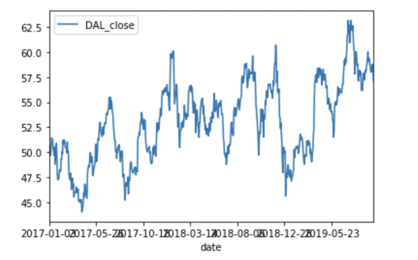
We can then visualize the data by running a simple:
delta.plot()And Voilà!
Creating a Label
As previously mentioned, since we are using supervised learning, we need a label in order to make predictions. For our label, we will be using the Delta stock price 20 days into the future for each entry in the DataFrame.
forecast = 20
delta['prediction'] = delta['DAL_close'].shift(-forecast)
The forecast value can be changed to reflect any time window.
Splitting the Data
A common convention when conducting a machine learning project is to set aside a testing set from the original data set. The purpose of a test set is validate the trained model on data instances that have not been seen. In order to split the training set and the testing set, I used the Sci-Kit Learn function train_test_split. Since we are working with time series data, it is important to make sure that the training set is shuffled to prevent unwanted bias.
The following step is not necessary, but can be considered good practice. First, we drop our label and then shift the training set to account for the forecast. Second, we assign our label to the y variable and shift by the forecast window. The Sci-Kit Learn function is called and 20% of the original data is set for testing.
X = np.array(delta.drop(['prediction'],axis=1))
X = X[:-forecast]
y = np.array(delta['prediction'])
y = y[:-forecast]
x_train, x_test, y_train, y_test = train_test_split(X, y, test_size=0.2)
Training the Models
As previously mentioned, for this project, we are focusing on two basic models for regression, a support vector machine and a linear regressor.
Support vector machines can be used for regression. When using support vector regression (SVR), decision boundaries are created around the input and a margin of tolerance (epsilon) is developed for making approximations. Sci-Kit Learn has an implementation for Support Vector Regression. Read more about it here.
A linear regression model makes a prediction by computing a weighted sum of the input features. A bias term is added to the tail of the linear model. Read about Sci-Kit Learn’s implementation here.
Below, we create the two models and then use the fit function to train the models on our input data.
svr_rbf = SVR(kernel='rbf', C=1e3, gamma=0.1)
svr_rbf.fit(x_train, y_train)

lr = LinearRegression()
lr.fit(x_train, y_train)
Rating the Models
There are several different types of metrics that can be used to evaluate the accuracy of a model. For this project, each of the models are evaluated using the score function. The score function returns the R² coefficient which evaluates the closeness of fit of the data points to the model. The highest value the R² score could be is one. As you will see, both of the models score relatively low. The low score can be attributed to the lack of correlation and the low amount of features used in training. We use the test set for scoring, because our models have not yet seen any of the test set data.
# Testing Model: Score returns the coefficient of determination R^2 of the prediction.
# The best possible score is 1.0
lr_confidence = lr.score(x_test, y_test)
svr_rbf_confidence = svr_rbf.score(x_test, y_test)
In order to obtain higher confidence scores, The hyper parameters of each of the models can be experimented with, also known as hyper parameter tuning. Another way to boost confidence scores is to introduce new features into the training data. In your own time, try finding a highly correlated stock to pair with the stock that you are trying to make predictions on.
… But always beware of overfitting!
Setting Up the Predictions
… Now for the fun part! If you have made it this far, thank you. Before we make our predictions we need to set up a separate array which will contain all of the dates for which we intend to make predictions.
# Set x_forecast equal to the last 20 rows of the original data set from Adj. Close column
x_forecast = np.array(delta.drop(['prediction'],axis=1))[-forecast:]
Predictions!
Below, we make predictions on our previously created array. We store the predictions in two separate variables.
lr_prediction = lr.predict(x_forecast)
svm_prediction = svr_rbf.predict(x_forecast)
Saving the Predictions
In order to plot the predicted values side by side with the actual values, we create two new columns in the original DataFrame. Our prediction values are then stored in the DataFrame.
delta['lr_pred'] = np.nan
delta['svm_pred'] = np.nan
delta.loc['2019-09-04' : '2019-10-01', 'lr_pred'] = lr_prediction
delta.loc['2019-09-04' : '2019-10-01', 'svm_pred'] = svm_prediction
Visualizing the Predictions
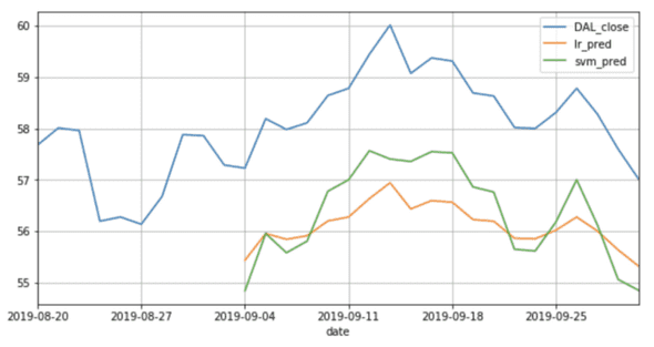
To visualize our results, we plot the actual values are our predicted values.
delta[-30:].plot( y=['DAL_close', 'lr_pred', 'svm_pred'], figsize=(10,5), grid=True)Through interpretation of the graph, it can be deduced that both of the predictions were similar. Initial values definitely varied from the actual. The regression models seemed to excel at predicting the trends but not the actual price values. Try running a cumulative sum based on the returns of the actual closing price and comparing it to the predicted price value cumulative return sum.
Conclusion
Although our regression models were not that accurate, hopefully this was a good starter to help familiarize you with some basic machine learning concepts. In the future, I will be creating more robust models and develop trading strategies, but it important to understand why machine learning is powerful and how it can be applied.


