Compare Stock Pairs for Your Algorithmic Trading Strategy with Quantopian
As I mentioned in my previous article, I have started using Quantopian for quantitative stock research. Following their lecture series has been informational, and the best part about their platform is that it is completely free to use.
In this article, I will be demonstrating a basic way to compare two different assets. The comparison of correlated assets has use cases in several trading strategies.
Pairs Trading
Pairs trading is one popular strategy that aims to utilize the correlation of two securities. Pairs trading is market neutral, meaning that it has the potential to benefit from positive or negative trends [1]. Pairs trading requires two highly correlated assets. It is important that the securities maintain their correlation because it is necessary for the execution of the strategy. In concise terms, a trader would take out a long position on one of the correlated assets that begins to underperform, and go short, simultaneously on the outperforming asset. The hope is that the two assets will eventually converge due to their strong correlation and the trader will benefit from both positions.
Although I will not be implementing a pairs trading algorithm, my objective is to lend you some code that can help you analyze the correlation between two assets.
Start Coding
All of the code for this article was written in a Quantopian Notebook environment. They have preinstalled several different packages which make it incredibly easy to focus on logic.
The chosen dates are arbitrary, but I prefer looking at a larger window. The assets, also arbitrary chosen by me, are two of the most liquid ETFs, the SPY and QQQ. The SPY aims to track the S&P 500, while the QQQ tracks the Nasdaq 100. Both are two of the most popular market indices. The get_pricing() function, provided by Quantopian, is a convenient way to access pricing information for the specified date fields. The function returns a data frame and the piece of code that follows restructures the column names, so that they are more accessible. Finally, the pandas head function is called to verify the returned data frame.
import pandas as pd
import numpy as np
import matplotlib.pyplot as plt
start = '2015-01-01'
end = '2020-05-30'
data = get_pricing(['SPY', 'QQQ'], fields='price', start_date=start, end_date=end)
data.columns = [e.symbol for e in data.columns]
data.head()Check Out Those Returns
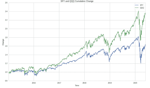
Before we waste our time trying to see if the assets are correlated, we can analyze the cumulative returns. There are several ways to verify the correlation, but it can’t hurt to look at the return potential and trends over our selected time period.
In order to visualize the cumulative returns, I created two new data frame columns that each use the pandas pct_change function. We then plot the cumulative product of those returns. Again, there are different ways to visualize return trends, but I prefer this way due to its simplicity. Finally, we utilize matplotlib to display the result.
data["SPY_PCT_CHANGE"] = data['SPY'].pct_change()
data["QQQ_PCT_CHANGE"] = data['QQQ'].pct_change()
plt.plot((data["SPY_PCT_CHANGE"] + 1).cumprod(), label="SPY")
plt.plot((data["QQQ_PCT_CHANGE"] + 1).cumprod(), label="QQQ")
plt.title("SPY and QQQ Cumulative Change")
plt.xlabel("Time")
plt.ylabel("Change")
plt.legend()
Wait it’s really that easy?
Up to this point if you are struggling with the Quantopian platform, I highly encourage you to checkout their tutorials, and brush up on the basics of matplotlib, pandas, and python. It will only help in the long run. Trust me, it only gets easier from here!
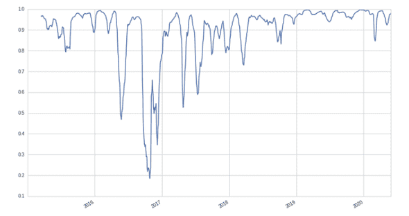
To calculate the correlation between the two securities, we need some data points. I chose a 50 day window using the pandas rolling function. After, finding the correlation is as easy as just using the word corr. Told you! It’s easy. From there, we plot for a visualization. From the graph below, it is clear the two ETFs share a high correlation for a majority of the time window. Try playing around with a different number in the rolling function.
data["SPY"].rolling(50).corr(data['QQQ']).plot();Conclusion
It is clear that the two assets maintain a strong positive correlation for a majority of the time window. For a pairs trading strategy, a correlation of 0.8 or greater is recommended. In my next article, I plan on introducing the Quantopian Algorithm environment. The Algorithm environment is where actual trading strategies are executed during backtests. A majority of my articles have been simplistic and focused on visualization, but the fun part is coming. I promise.
Sources
[1] https://www.investopedia.com/articles/trading/04/090804.asp


