Buy and Hold vs. Moving Average Crossover, and a Gentle Intro to Quantopian
Recently, I have started working on Quantopian. Quantopian is an excellent website that provides free financial data and educational resources for aspiring quantitative analysts. Most of my previous work was completed in a local Python environment, but the Quantopian platform has a great collection of resources for prototyping new strategies.
If you haven’t heard of Quantopian, consider this article an introduction. I highly recommend checking out their tutorials and lectures for more in depth explanations. Their software is incredibly easy to use and is very powerful. In the future, I plan on using Quantopian for backtesting my ideas, in order to validate my assumptions. Quantopian provides an environment for rapidly prototyping ideas, without requiring quants to set up a robust environment for themselves.
Getting Started
Consider this article a gentle introduction to the platform. In subsequent articles, I plan on covering some of the other features of the platform because finding a soft place to start can be daunting. The code that follows can all be easily run in the Notebook tab on Quantopian, all you need to do is create an account. Everything else is FREE! … a rarity in the world of financial data.
With Quantopian, you don’t need to worry about installing any of the commonly used Python packages. They have take the time to do that for you. If it seems too good to be true, it isn’t. It’s that easy.
For this article, I will highlight how easy it is to implement a buy and hold strategy based on moving averages.
Now for Some Code
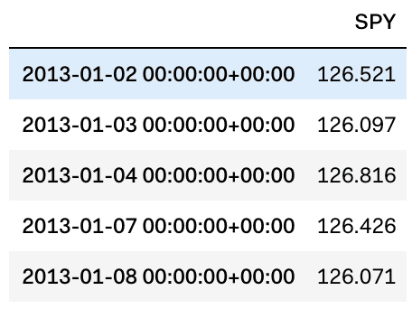
First, we start by importing the necessary packages. Pandas for data manipulation, numpy for working with arrays, and matplotlib for graphing. In order to pull price data for a security, I used a function provided by Quantopain called get_pricing(), which is pretty self-explanatory. The function returns a pandas data frame of the price data for each day for our selected security, the SPY. The SPY is an ETF that tracks the S&P 500 index. We then call the pandas head function to look at the first 5 rows of the returned data frame.
import pandas as pd
import numpy as np
import matplotlib.pyplot as plt
start = ‘2013–01–01’
end = ‘2020–05–30’
data = get_pricing([‘SPY’], fields=’price’, start_date=start, end_date=end)
data.columns = [e.symbol for e in data.columns]
data.head()
The Strategy
When trading a moving average crossover, the strategy says to go long when the shorter average crosses over the longer average to the upside. When the shorter average crosses back over the longer average to the downside, we sell. In some cases, a short might be used, but for sake of simplicity, we will just sell out of the previous position.
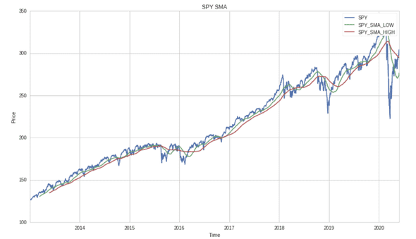
Below, I calculate both of the moving averages. In this case, I considered a 50 day moving average and a 100 day moving average. The lengths are arbitrary and can be experimented with. We then plot the two averages alongside the pricing data provided by Quantopian, in order to visualize and juxtapose their differences.
data["SPY_SMA_LOW"] = data['SPY'].rolling(50).mean()
data["SPY_SMA_HIGH"] = data['SPY'].rolling(100).mean()
plt.plot(data["SPY"], label='SPY')
plt.plot(data["SPY_SMA_LOW"],  label="SPY_SMA_LOW")
plt.plot(data["SPY_SMA_HIGH"],  label="SPY_SMA_HIGH")
plt.title("SPY SMA")
plt.xlabel("Time")
plt.ylabel("Price")
plt.legend();
Following the strategy, when the smaller window moving average is greater than the larger, we buy, or take a position of 1, indicating a buy. When the smaller window moving average falls below the larger one, we sell, or take a position of 0. In order to create the position, I created a new column in the data frame corresponding to each trading day. Using the numpy where function, I provided the necessary expression logic that evaluates to 1 if true, signaling a buy, and 0 if false, indicating a sell.
data["Position"] = np.where(data["SPY_SMA_LOW"] > data["SPY_SMA_HIGH"], 1,0)Calculating Returns
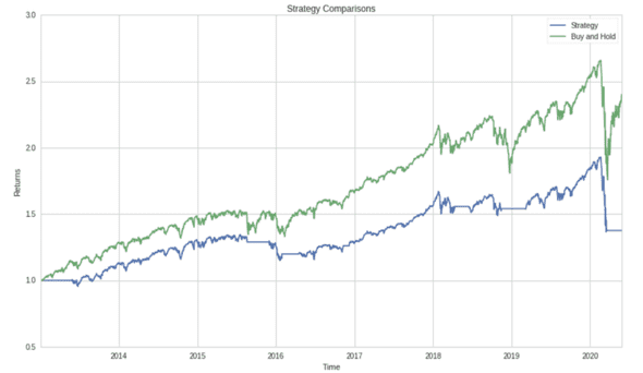
In order to measure returns, we first need to shift the position column in order to reflect accurate intake of the data. The column is shifted because we would be making the trade a day after the crossover occurs, as we are not predicting the crossover. We are merely observing it. For days we buy, we assign a new column with the percentage change of the SPY for that day. To measure returns, we create individual columns for the strategy and compare them with buying and holding the security. The cumprod function finds the cumulative product of the data frame’s respective column. Finally, we plot the results.
data["Position"].shift()
data["StrategyPct"] = data["SPY"].pct_change(1) * data['Position']
data["Strategy"] = (data["StrategyPct"] + 1).cumprod()
data["BuyHold"] = (data["SPY"].pct_change(1) + 1).cumprod()
plt.plot(data["Strategy"], label='Strategy')
plt.plot(data["BuyHold"],  label="Buy and Hold")
plt.title("Strategy Comparisons")
plt.xlabel("Time")
plt.ylabel("Returns")
plt.legend()
Conclusion
Trading a moving average crossover, might not be the best idea. The flatlines indicate a sell position, where we are not long on the SPY. From observing the graph, it is clear that some days with rather large returns are missed. Don’t be discouraged! Although this strategy, won’t make you a millionaire, you can now use Quantopian… or at least the research environment.
As I mentioned before, in future posts, I will talk about using the algorithm environment, how to backtest ideas, and how to analyze your strategy before you waste time figuring out if it’s worth pursuing. Stay tuned, and thank you for reading!
Quantopian API Docs: https://www.quantopian.com/docs/api-reference
All code photos are screenshots from the Quantopian Platform


